Introduction

I’ve recently read this old blog post by Andrej Bauer about Martin Escardó’s Infinite sets that admit fast exhaustive search. At first, it seems pretty ridiculous! How is it possible to decide a problem that is embedded in an infinite topological space? However, using some nice tricks from functional programming and higher-level computability, we can achieve this and even explore some other unexpected consequences.

Any finite set is immediately exhaustible¹, but the interesting thing is that certain infinite sequences with specific properties can also be exhaustible.

Notation

The simple types are \sigma, \tau := o | \iota | \sigma \times \tau | \rightarrow \tau. Let’s dig into this a bit more. - o the Booleans which in Haskell are Bool = True | False - \iota (natural numbers), written as Int. - Product type \sigma \times \tau is the Cartesian product, which is IntMap a : \tau \times (Maybe a) - Function type \sigma \rightarrow \tau - \iota \rightarrow o = predicates on the naturals - o \rightarrow o = boolean functions \neg, \land, \lor, etc.

Using these primitives, we can construct increasingly more complex types as:

Base case (level 0): - o = booleans - \iota = natural numbers

Level 1: - o \times o = pair of booleans (True, False) - \iota \times \iota = pair of naturals (3, 7) - o \rightarrow o = boolean functions {NOT, AND True, OR False, id, ...} - \iota \rightarrow o = predicates on naturals {isEven, isPrime, λn.n>5} - \iota \rightarrow \iota = arithmetic functions, {successor, λn.2*n, λn.n²}

type Oracle a = Int -> a        -- ι → a (where a could be o, ι, etc.)
type Pred a = Oracle a -> Bool  -- (ι → a) → o  
type Prefix = IntMap Bool        -- finite partial assignments  

• The domain is a Cantor space \mathbb{B}^\mathbb{N} (all boolean streams)
• A predicate p is a higher-type functional p: (\mathbb{B}^\mathbb{N}) \rightarrow \mathbb{B}
• a prefix asg is a finite partial map \alpha : S \rightarrow \mathbb{B} which is used to define the cylinder sets used to define the product topology on the Cantor space. ### Scott Domains For each type \sigma, there is a Scott domain D_\sigma of partial functionals of the that same type \sigma defined by lifting the type \sigma to contain the undefined type with all of the properties you would expect (e.g. ordering, etc.). In Haskell, this looks like an Oracle a type with potential Need exceptions. This lets us capture the behavior of undefined/non-terminating computation, which we use to create partial oracles.

Total functionals T_\sigma \subseteq D_\sigma

A functional is total if it maps total inputs to total outputs (so it never produces a Nothing type from non-Nothing)

evalP :: Pred a -> Prefix a -> Either Int Bool
evalP p asg = case unsafePerformIO (try (evaluate (p (oracle undefined asg)))) of
  Left (Need i) -> Left i    -- Partial: needs position i
  Right b -> Right b         -- Total on this prefix

So then we can evaluate P(f^\perp) where f^\perp is a partial oracle depending on what the domain is.

Constructive Selection Functional for Cantor Space

Now consider the following code:

escardo :: Pred -> Maybe Oracle
escardo p = fmap extend (go IM.empty) where
  extend asg i = IM.findWithDefault False i asg
  go asg = case evalP p asg of
    Right True  -> Just asg
    Right False -> Nothing
    Left i -> case go (IM.insert i False asg) of
      Just a  -> Just a
      Nothing -> go (IM.insert i True asg)

We maintain a finite assignment asg that fixes the values of a few coordinates so far. evalP determines whether this cylinder already forces the truth value of p. If evalP p asg returns Right True, then p is already true for every infinite bitstream extending asg. Then we can just stop and produce a total oracle by calling extend, which fills every unspecified bit (at this current point) with a default value (False).

But what does this mean? Think of the Cantor space as the set of all infinite binary sequences

000000000... \\ 001010110... \\ 010101010... \\ 111111111... \\

From Wikipedia, > Given a collection S of sets, consider the Cartesian product X = \Pi_{Y \in S} Y of all sets in the collection. The canonical projection corresponding to some Y \in S is the function p_Y : X \rightarrow Y that maps every element of the product to its Y component. A cylinder set is a preimage of a canonical projection or finite intersection of such preimages. Explicitly, we can write it as: \bigcap_{i = 1}^n p_{Y_i}^{-1} (A_i) = \{(x) \in X | p_{Y_1} \in A_1, \cdots, p_{Y_n} (x) \in A_n \}

So for the Cantor space, a cylinder [\alpha] consists of the set of all infinite strings that start with a finite prefix \alpha. For example, - [01] = all strings that start with “01”: 01000000... \\ 01001010... \\ 01010101... \\ 01111111... \\ - [101] = all strings starting with “101”: 10100000... \\ 10101010... \\ 10111111... \\

We can illustrate this as a tree:

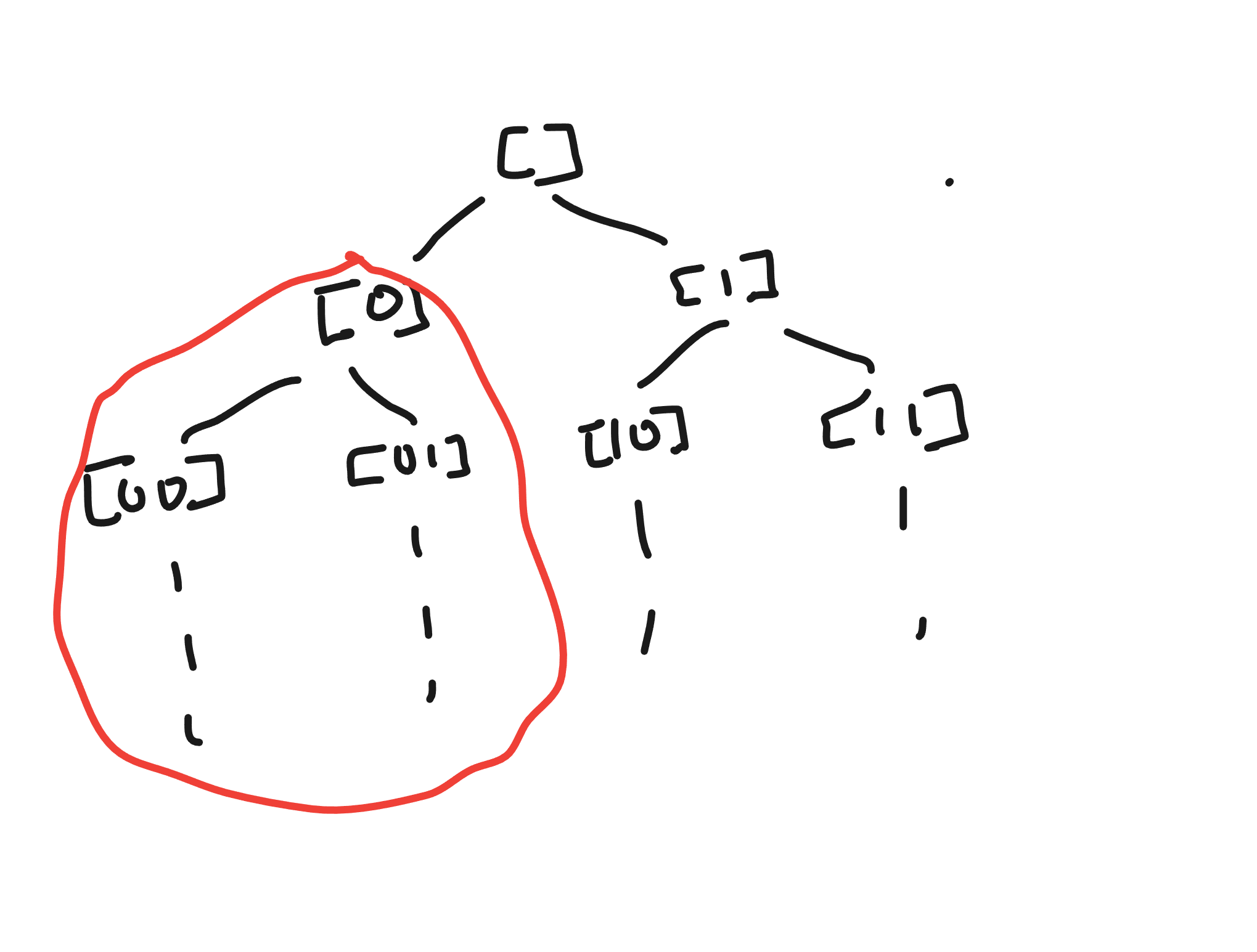The cylinder set corresponds to the subtree circled in red in the case of the Cantor space.

So then, the search process starts at the root and recursively tries to decide p on the current space (starting with the entire Cantor space). If we need bit i, then split the current cylinder into two subcylinders. If a cylinder returns Right False, we abandon the subtree and if a cylinder returns Right True, we short-circuit and accept.

The incredible thing is that predicate p in this case can be incredibly general. The simplest form to imagine are SAT-style boolean combinations, but they can be any continuous function decidable with finite information. For instance, all of the following are compatible with this framework and are decidable efficiently:

-- Arithmetic predicate
sumFirst10 :: Pred Int  
sumFirst10 oracle = sum [oracle i | i <- [0..9]] > 50

-- Pattern matching
hasPattern :: Pred Bool
hasPattern oracle = any (\i -> oracle i && oracle (i+1) && not (oracle (i+2))) [0..97]

-- Convergence predicate  
converges :: Pred Double
converges oracle = abs (oracle 100 - oracle 99) < 0.001

and these aren’t easily expressible using an SAT-style alphabet. The key constraint is continuity, not logical structure.

for the sake of mathematical rigor

Recall that formally, the predicate is defined as p: \mathbb{B}^\mathbb{N} \rightarrow \mathbb{B} a continuous map on the Cantor space, which itself is a countable product space. The basic open sets in this space are the aforementioned cylinders [\alpha], which are infinite bitstreams that extend a finite assignment \alpha : S \rightarrow \mathbb{B}. By the (Kleene-Kreisel) continuity of p, there exists some cylinder [\alpha] \ni x for each x on which p is already constant and hence a finite amount of information about the input fixes the output. Because the Cantor space is compact and totally disconnected, the preimages p^{-1} (1) and p^{-1} (0) are clopen, so each can be written as a finite union of cylinders (this is a pretty standard trick). Refining these finitely many cylinders to a common depth yields a uniform modulus² (via Heine-Cantor) N such that for each x, p(x) is determined by some finite set of at most N bits.

The evalP function implements this. Given a finite assignment alpha (the IntMap), we run p against the partial oracle that answers exactly the bits in \alpha and throws Need when an unassigned bit is requested. This is exactly the “dialogue” that Escardó describes in his paper: continuous higher-type functionals consuming only finite information..

So really, this is just an incredibly complex guided depth-first search over the binary decision tree of finite assignments that branches only when p asks for a new bit with some short-circuiting logic. Termination relies on compactness via the uniform modulus N. Left i can appear only when i is new (once a bit is assigned, accessing it later doesn’t throw a Need). Thus, no successful branch can be longer than N, so after at most N distinct queries continuity forces a Right answer. If p is everywhere false, the algorithm will explore all finitely many branches up to depth N and fail and otherwise terminate early. Thus, we constructively determine that the Cantor space is searchable³. Another nice property of this is that the order that we sample branches doesn’t affect correctness, only runtime (so there are many engineering optimizations to be done…maybe Gray codes?).

The TL;DR is that: - Continuity gives you cylinder-faithfulness - Compactness gives you a uniform finite modulus - Dialogue gives you an on-demand DFS that decides the predicate over finite information

why just the cantor space?

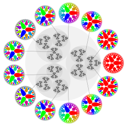Good ol’ Wikipedia image. Unfortunately took me a few months to fully wrap my head around them.

The p-adic integers⁴ \mathbb{Z}_p can similarly be seen as an infinite stream of digits in the base p much like the Cantor space (as shown above).

x = a_0 + a_1p + a_2 p^2 + \cdots, a_i \in \{ 0, 1, \cdots, p - 1 \}

Really, the only difference is that now the alphabet size is now p instead of restricted to 2. The Cantor space is kind of an artificial playground because conceptually it is pretty simple to understand. However, the p-adics are widely applicable across number theory (Hensel’s lemma always surprises me) and more. We can easily compute the answer for the question “does there exist a p-adic number \geq k that satisfies C condition?” and construct a witness for it. At some point, i’ll implement a root finding constructive algorithm…maybe pure Haskell WolframAlpha??

There is also an extension of this that introduces Randomness and in turn has some interesting measure-theoretic and algorithmic properties..