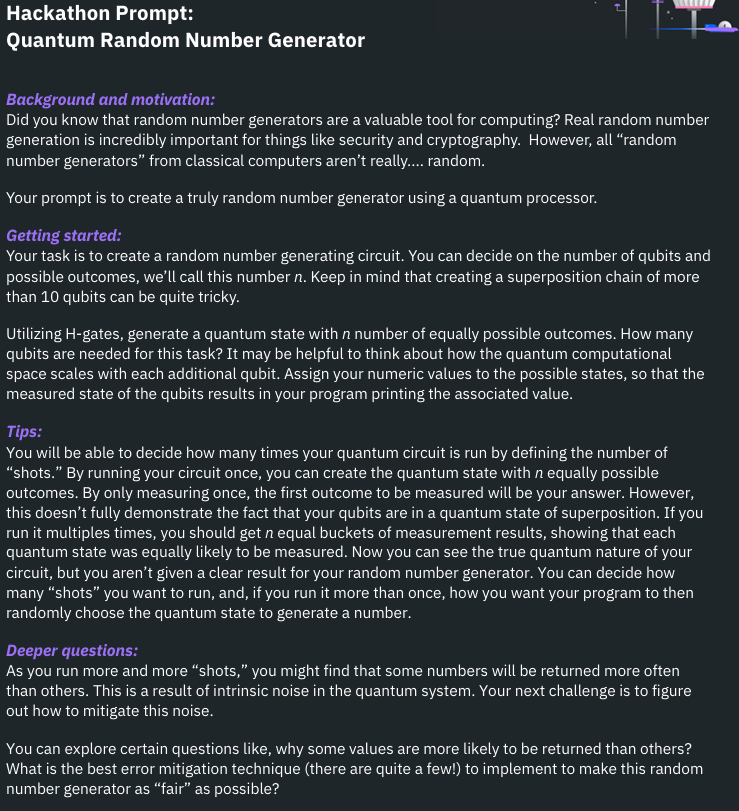
Quantum Random Number Generator

October 19, 2025 • #quantum

First time trying anything quantum computing w/ my friend Shuhul from Caltech :)

Prompt

In this project for QiskitFest@UCLA, we implement a Quantum random number generator that uniformly samples $0...N$ in the fewest number of qubits and gates as possible. We include 4 sample circuits ranging from a naiive implementation to the most optimal design.

Preliminaries:

Quickly, this problem of sampling $0..N$ is trivial for the case $N = 2^k$, since we can use a series of Hadamard transforms to evenly split the amplitudes across all $2^k$ computational basis states. Each Hadamard gate doubles the number of possible outcomes, creating a uniform superposition where every basis state has equal probability $1/2^k$. This only becomes interesting when $N$ isn’t just a power of $2$, for which we explore a series of circuit constructions. Naiively, we could just simulate extra states and use rejection sampling, but we wanted to design this circuit to operate purely on a quantum state.

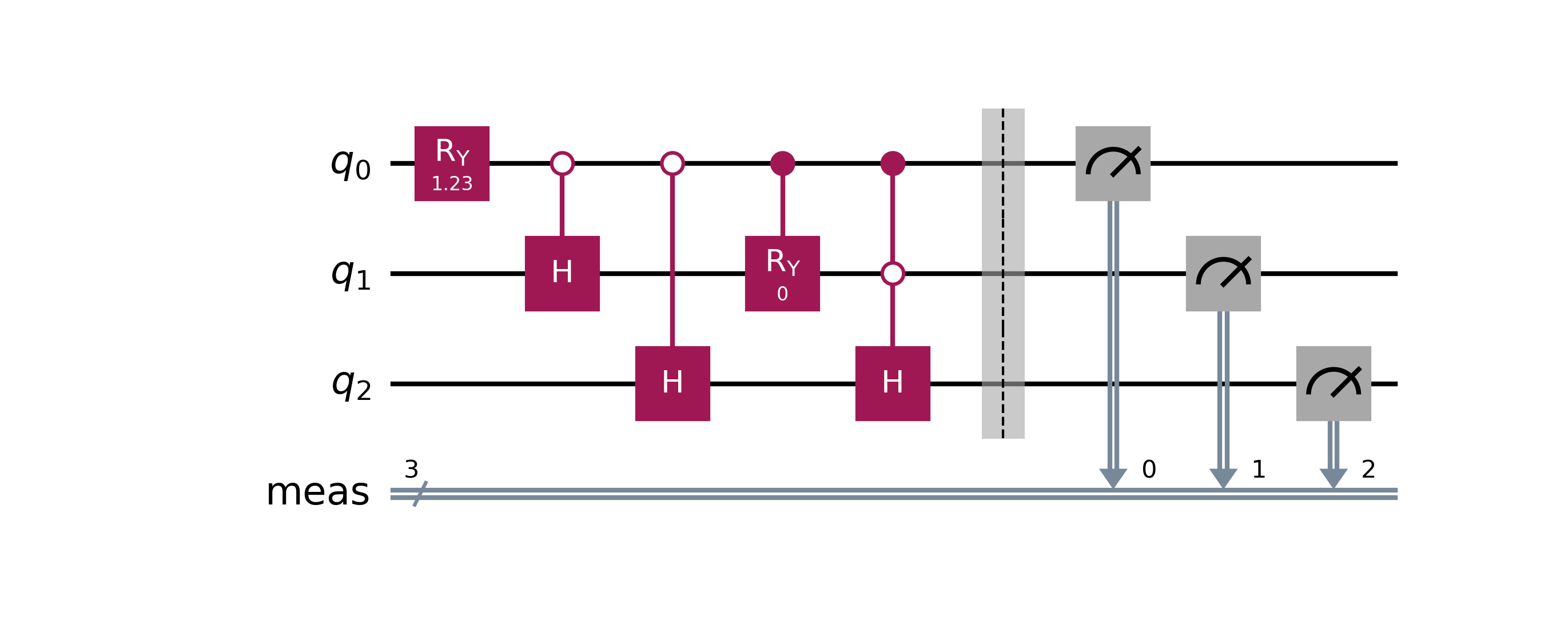
V0: Naiive Control

In this circuit, we manually set the probabilities of each qubit using cascaded $R_y$ rotations, but this approach quickly becomes impractical. Each new qubit requires multiple controlled rotations whose angles depend on all previous qubits, causing the gate count and circuit depth to grow quadratically. These controlled rotations are also error-prone and hardware-expensive, and the precise rotation values are hard to compute or calibrate.

V1: Binary Expansion

Since for powers of 2, building a uniform sampler is straightforward using Hadamard gates, we instead view $N$ as a sum of powers of two, $N = 2^{k_1} + 2^{k_2} + \cdots + 2^{k_m}$. By constructing uniform superpositions for each $2^{k_i}$ block and combining them with conditional rotations, we can approximate a uniform distribution over $0...N-1$ while keeping the circuit shallow and efficient.

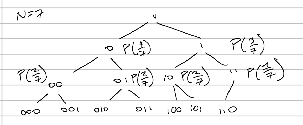
Example

Here is an example of the breakdown for $N = 7$:

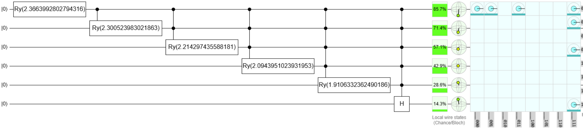
And here is the corresponding circuit representation

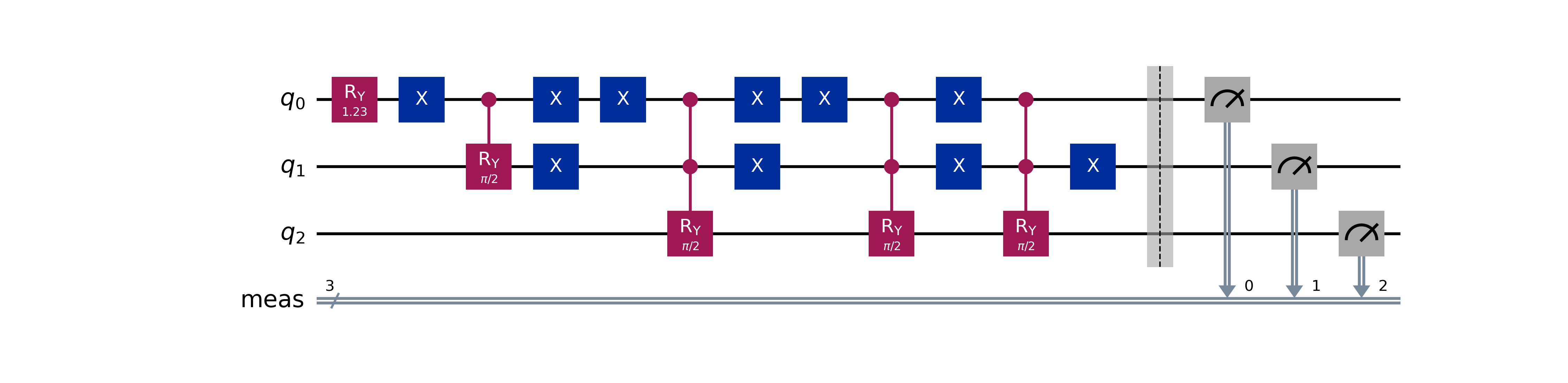
We recursively sample over $N = 7$ states as a binary tree of conditional probabilities. At each branching point, the circuit applies a rotation that splits the amplitude proportionally to how many valid states remain in each subtree.

For instance, the first qubit has probability $P(4/7)$ of being $|0\rangle$ and $P(3/7)$ of being $|1\rangle$. These are then recursively refined until all of the basis states are assigned equal amplitude.

Some Math

For the first qubit, we want to split the probability mass between the left and right branches according to how many valid states lie under each.

$$P(0) = \frac{4}{7}, \quad P(1) = \frac{3}{7}.$$

An $R_y(\theta)$ gate on $|0\rangle$ prepares

$$R_y(\theta)|0\rangle = \cos\left(\frac{\theta}{2}\right)|0\rangle + \sin\left(\frac{\theta}{2}\right)|1\rangle,$$

giving probabilities $\cos^2(\frac{\theta}{2})$ and $\sin^2(\frac{\theta}{2})$. Setting $\cos^2(\frac{\theta}{2}) = \frac{4}{7}$ yields

$$\boxed{\theta = 2\arccos\sqrt{\frac{4}{7}} = 2\arcsin\sqrt{\frac{3}{7}}.}$$

V2: Consolidating Hadamards

Since the Hadamard gate is unitary, applying it twice yields the identity operation $H^\dagger H = I$. Previously, we used a Hadamard gate with a control to emulate an anti-control, but since H is self-inverse, we can simplify the circuit by directly using an anti-control instead, reducing unnecessary gates.

V3: Complement Graph

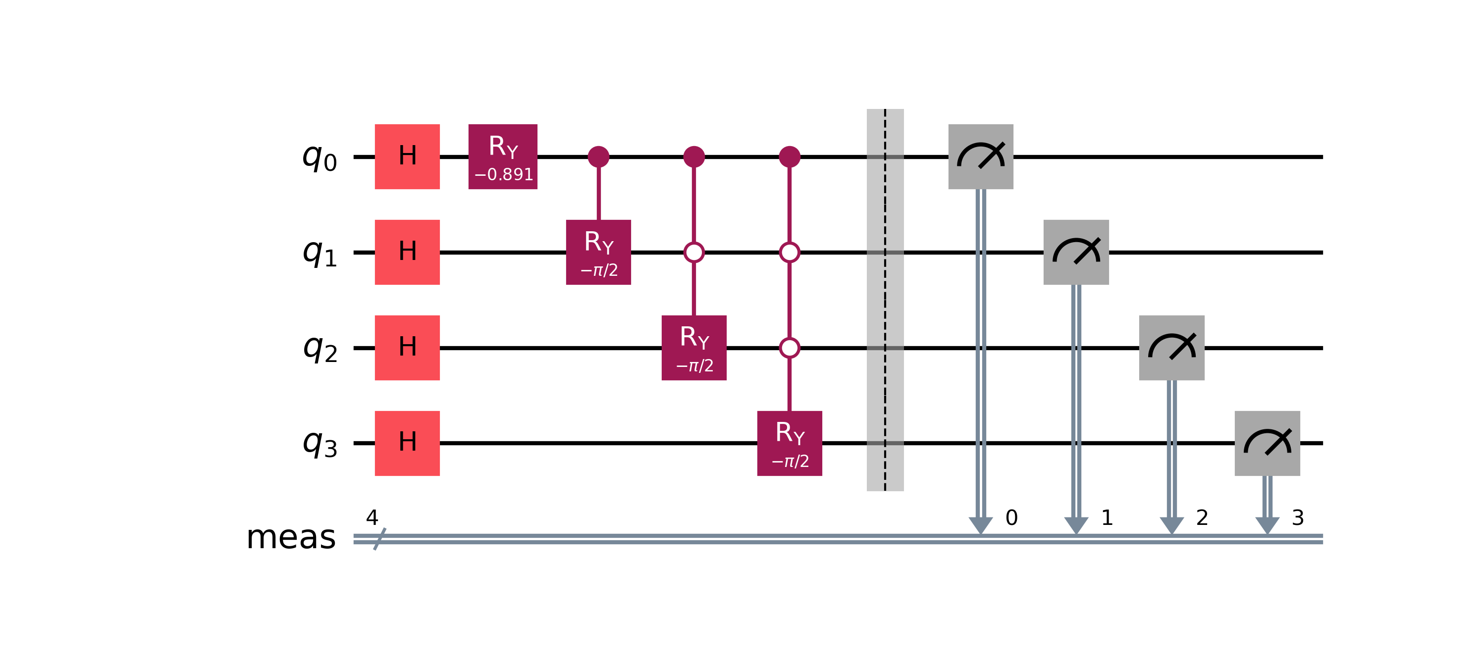
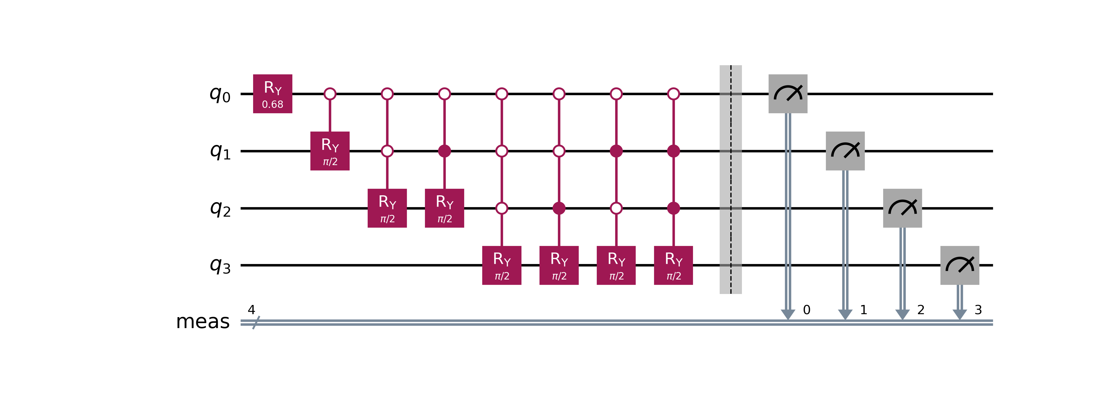
This approach first builds a fully balanced superposition over $2^k$ states using Hadamard gates, then applies conditional $R_y$ rotations to correct the amplitudes for $N < 2^k$. The Hadamard layer creates an even base distribution, while the correction step prunes invalid branches, creating an even more compact circuit.

Example

For $N=9$, where the first split is $N_0=8$ and $N_1=1$, the rotation angle is

$\theta = 0.680 \text{ rad},$

so relative to a Hadamard baseline ($\pi/2$), the correction is

$\Delta\theta = -0.891 \text{ rad}.$

V4: Log-depth Hadamard Expansion

To build a uniform quantum state over $0 \ldots N-1$, we basically follow the binary expansion of $N$. Each power of two, $2^j$, is like a “block” of evenly distributed states, and you only need $j$ Hadamards to generate it, since each Hadamard doubles your reach. So if $N=9=8+1$, you use three Hadamards to cover the first eight states and then just patch in the last one. The key idea is that you don’t brute-force all $N$ outcomes — you reuse the structure of powers of two to get there in about $\log N$ steps, with a few small corrections at the end to make everything line up perfectly.

There might be a slightly more clever way of reducing the number of control gates, but this is the best we could do up to gates and number of qubits.

Exercise (for fun)

Let $k = \lceil \log_2 N \rceil$ and $D = 2^k - N$.

Estimate when the complement approach (cost $O(D)$) becomes less efficient than the Hadamard tree method (cost $O(\log N)$).

← Back to posts